Playing With K-nearest Neighbors Algorithm

k-Nearest Neighbors is the algorithm that barely deserves the name. It doesn’t train; it doesn’t fit parameters; it doesn’t build a model. It just remembers every labeled example, and when you hand it a new point it finds the k closest ones it has seen and lets them vote. That’s the whole idea — and yet, exactly because it’s so transparent, kNN is one of the best lenses I know for thinking about the questions that haunt every classifier: how much should a model trust its neighbors, where do you draw the line, and how do you know your accuracy isn’t a lie?

(One terminology note up front, since the original version of this post got it wrong: kNN classification is supervised learning — it relies on labeled examples. The unsupervised cousin, k-means, is a different animal entirely.)

So I built a small kNN classifier over a two-dimensional dataset and studied how its two dials — the number of neighbors k and the decision threshold — change its behavior, validated three different ways.

A query point takes the majority label of its k nearest neighbours — k is a bias/variance dial.

The algorithm, in a handful of lines

The core is almost insultingly simple: measure the distance to every stored point, keep the nearest k, and take a (thresholded) vote.

def classify(point, training, k, boundary):
    # rank every labeled example by Euclidean distance to `point`
    nearest = sorted(training, key=lambda p: distance(point, p))[:k]
    # fraction of those neighbors that are positive
    score = sum(1 for n in nearest if n.label == "positive") / k
    return "positive" if score >= boundary else "negative"

Two parameters fall out of that snippet, and the entire study is about what they do. k controls how many voices get heard; boundary controls how big a majority you demand before calling a point positive.

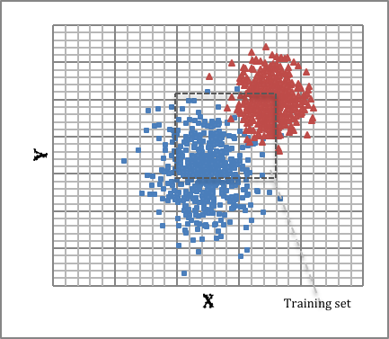
The dataset: positives cluster in the first quadrant, negatives in the third.

The data is deliberately tidy — positives sit mostly in the first quadrant, negatives in the third — with one telling asymmetry: a few negative points leak into the positive region, but almost no positive points stray into the negative one. That lopsidedness drives everything that follows.

k is a bias–variance dial

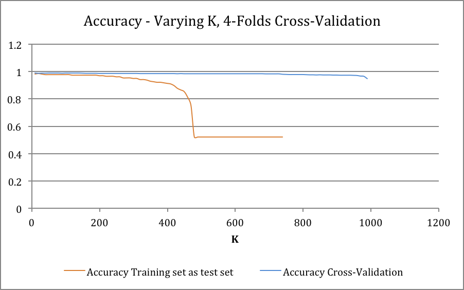
The number of neighbors is the cleanest illustration of the bias–variance trade-off in all of machine learning. A tiny k (say 1) gives an exquisitely flexible, jagged decision boundary that contours around every point — low bias, but high variance, and exquisitely sensitive to noise. A large k averages over a wide neighborhood, smoothing the boundary into something stable but blunt — high bias, low variance. Crank k high enough and every query just sees the majority class.

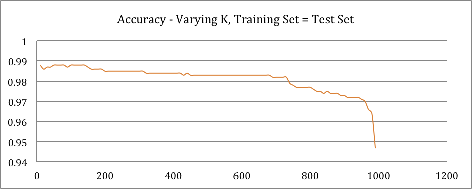
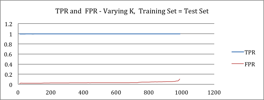
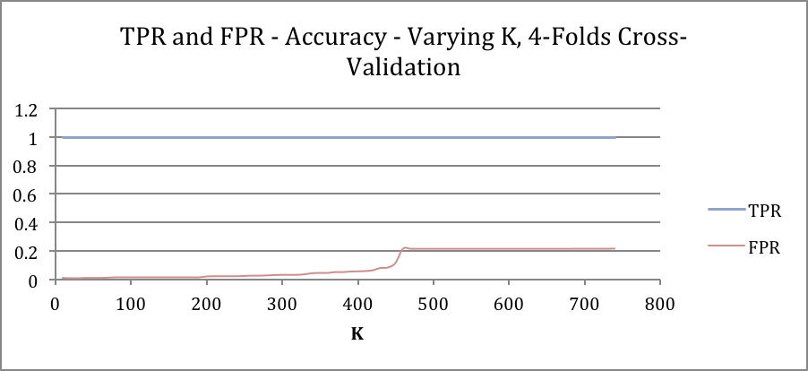
Accuracy declines as k grows — the neighborhood blurs past the useful scale.

The true-positive rate holds steady while the false-positive rate climbs with k.

Here’s where the dataset’s asymmetry shows up. As k grows, false positives rise faster than false negatives: the negative points that wandered into positive territory are surrounded by positives, so a wide vote happily mislabels them. The tightly packed positive cluster, by contrast, is barely perturbed. Geometry, not magic.

The decision threshold: optimism vs. pessimism

The boundary is the probability cutoff for declaring a point positive, and it is a pure precision/recall lever. Lower it and you become optimistic — you catch more true positives but also wave through more false ones. Raise it and you turn cautious, trading recall for precision.

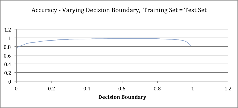
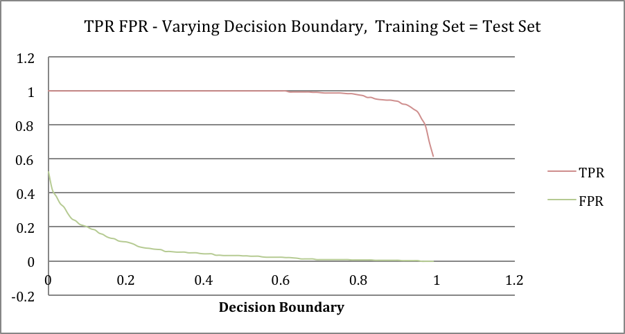
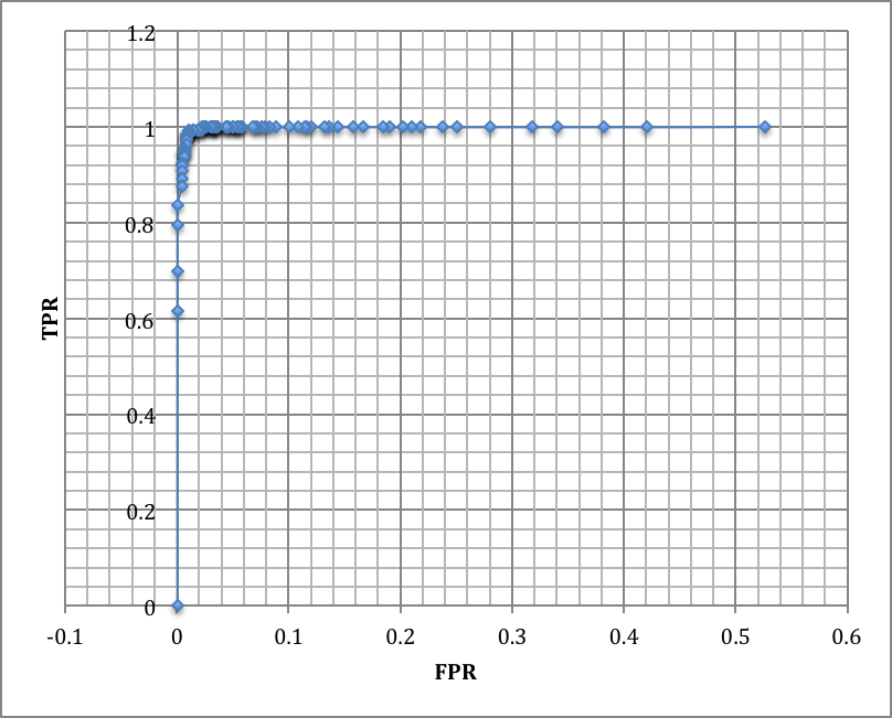
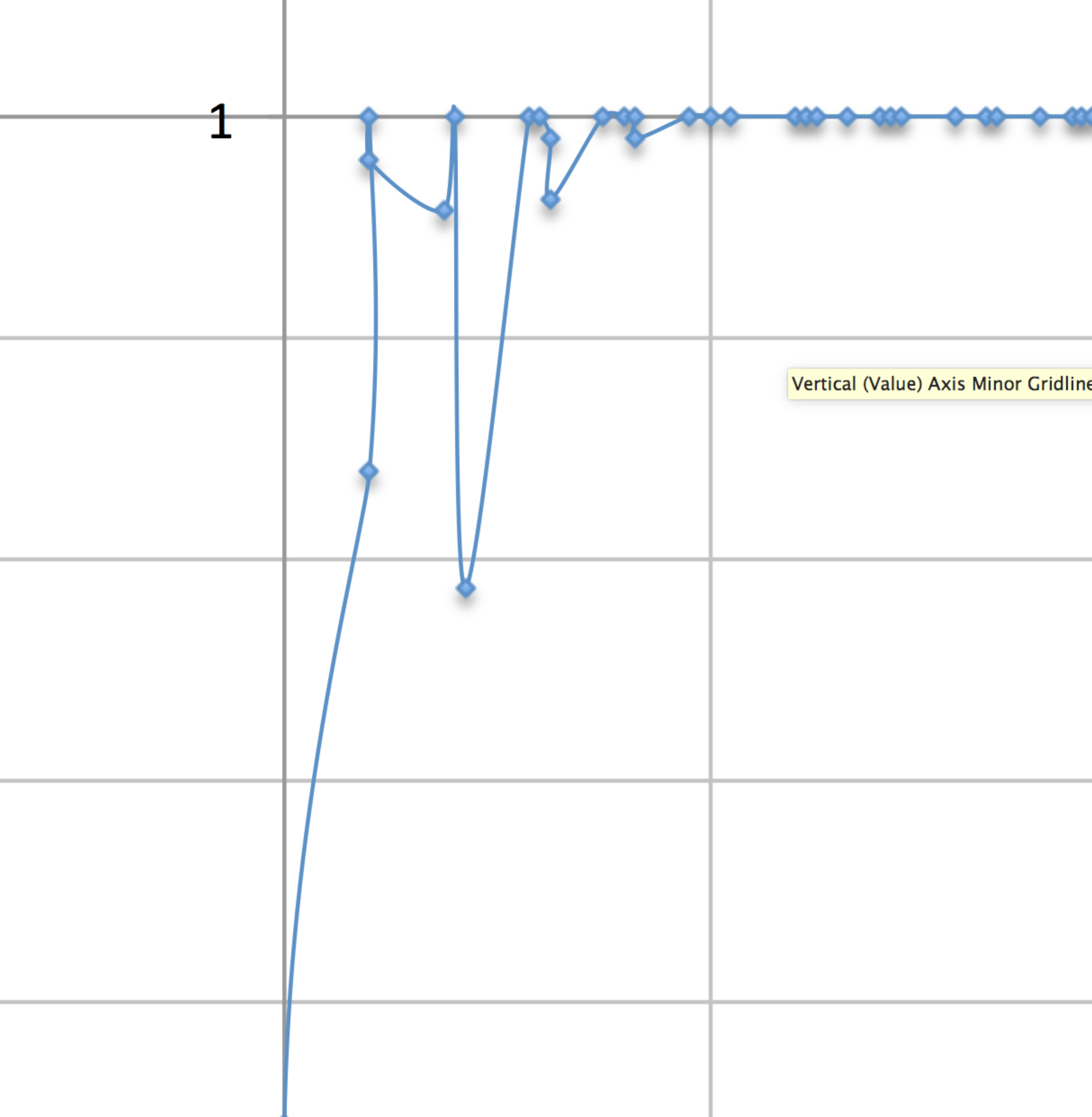
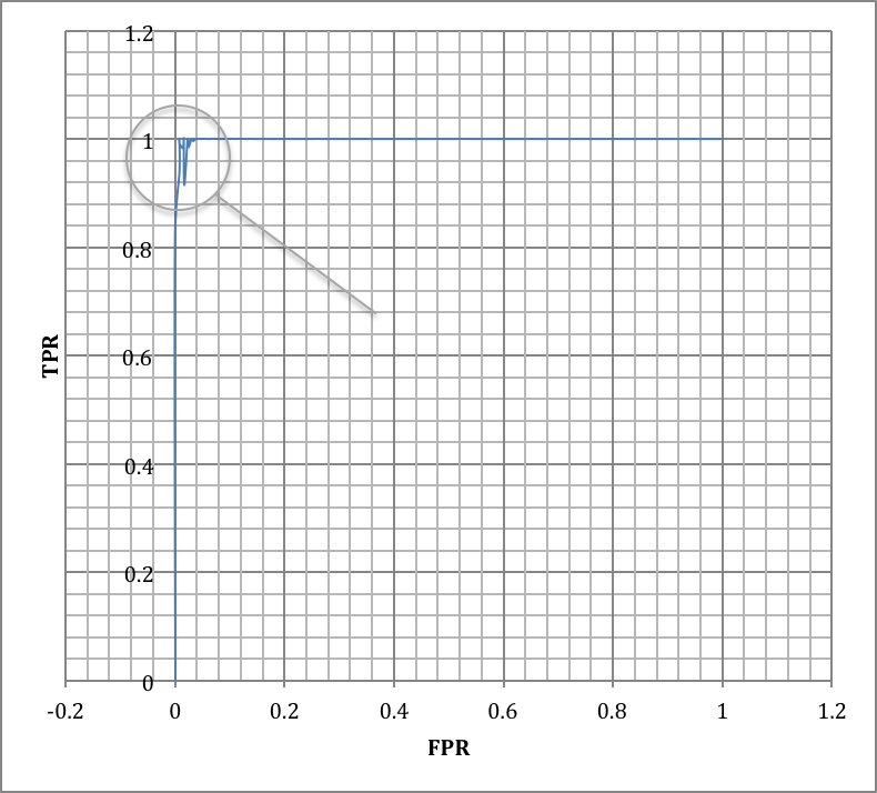
Accuracy versus decision boundary traces a downward parabola — the extremes are bad, a middling threshold is best.

As the threshold rises, the true- and false-positive rates both fall.

The accuracy curve over the threshold is a downward parabola: both extremes are poor and a moderate cutoff wins, which is exactly what you’d hope for. Sweeping the threshold from 0 to 1 and plotting the true-positive rate against the false-positive rate traces the ROC curve, and the area under it (AUC) is the threshold-independent summary of how well the classifier separates the classes.

The ROC curve hugs the top-left corner: a near-perfect classifier on this dataset.

Trust, but cross-validate

A near-perfect ROC is thrilling until you remember how it was measured. Scoring a classifier on the same data it learned from is the original sin of machine learning — it measures memorization, not generalization. The honest approach is k-fold cross-validation: shuffle the data, split it into folds, and repeatedly train on all-but-one fold and test on the one held out, so every point is predicted exactly once by a model that never saw it.

Cross-validation yields a more realistic, slightly humbler accuracy curve.

A sharp jump in the false-positive rate appears around k ≈ 450.

The cross-validated ROC stays excellent but now shows honest fluctuation.

The worst case: forcing it to extrapolate

Cross-validation estimates the average case. To find the floor, I rigged a deliberately cruel split: train only on the inner core of the data and test on the outer ring. That forces the classifier to extrapolate beyond the region it learned, which is precisely where nearest-neighbor methods are weakest — there are no near neighbors out there to ask.

Train-on-the-core, test-on-the-edges: the lowest AUC the dataset will give up.

What the experiment actually shows

Three lessons survive the graphs. First, k is a bias–variance knob and the best value lives in the middle, not at either extreme. Second, the decision threshold is an independent precision/recall knob, and accuracy over it is a parabola with a comfortable optimum. Third — and most importantly — the headline number depends entirely on how you measure it: training-on-test flatters, cross-validation tells the truth, and a worst-case split tells you how bad things get when the model is asked to leave home. A near-perfect ROC says as much about how separable this particular dataset is as it does about kNN. The algorithm that doesn’t really learn turns out to be a wonderful teacher.